Documentation for the integrals module

This module integrals defines all the integration functions required for the project. Below is included an auto-generated documentation (from the docstrings present in the source file).

---

Implementation of several algorithms for numerical integration problems.

• I was mainly interested about techniques to numerically compute 1D definite integrals, of the form \(\int_{x=a}^{x=b} f(x) \mathrm{d}x\) (for \(f\) continuous).
• Some functions can be used to plot a graphical representation of the technic (Riemann sums, trapez rule, 1D Monte-Carlo etc).
• There is also a few 2D techniques (Monte-Carlo, but also one based on Fubini’s Theorem), for integrals of the forms \(\displaystyle \iint_D f(x, y) \mathrm{d}x \mathrm{d}y = \int_{x=a}^{x=b}\left(\int_{y = g(x)}^{y = h(x)} f(x) \mathrm{d}y \right) \mathrm{d}x.\)
• Similarly, I experimented these two techniques for a generalized \(k\)-dimensional integral, inspired from this very good Scipy package (scikit-monaco) and scipy.integrate.
• Date: Saturday 18 June 2016, 18:59:23.
• Author: Lilian Besson for the CS101 course at Mahindra Ecole Centrale, 2015.
• Licence: MIT Licence, © Lilian Besson.

Examples

Importing the module:

>>> from integrals import *

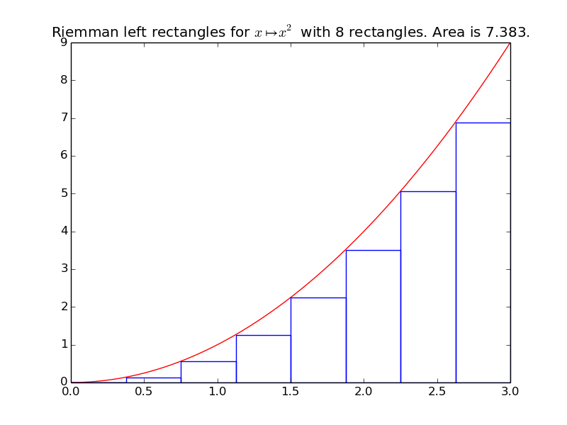
Let us start with a simple example \(x \mapsto x^2\), on \([x_{\min}, x_{\max}] = [0, 3]\).

>>> k = 2; xmin = 0; xmax = 3
>>> f = lambda x: x**k

We can compute formally its integral: \(\int_{x=a}^{x=b} f(x) \mathrm{d}x = \left[ F(x) \right]_{x_{\min}}^{x_{\max}} = F(x_{\max}) - F(x_{\min}) = \frac{3^3}{3} - \frac{0^3}{3} = 27/3 = 9\)

>>> F = lambda x: x**(k+1) / float(k+1)
>>> F(xmax) - F(xmin)
9.0

Riemman sums

Left Riemann sum, with 8 rectangles, give:

>>> riemann_left(f, xmin, xmax, n=8)  
7.382...

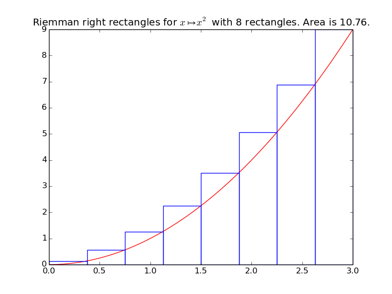
>>> riemann_right(f, xmin, xmax, n=8)  
10.757...

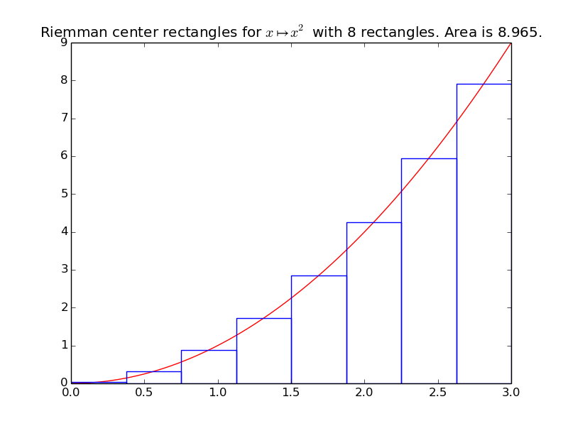
>>> riemann_center(f, xmin, xmax, n=8)  
8.964...

Trapezoidal rule

>>> trapez(f, xmin, xmax, n=3)
9.5

More examples

See below, at least one example is included for each integration method. Currently, there is 228 doctests, corresponding to about 50 examples of numerically computed integrals. (and they all pass, ie each test does exactly what it I expected it to do)

---

Small things that still need to be done

Todo

Conclude this main module: more Gaussian quadratures?

Todo

Make a general nd_integral() function, letting the user chose the integration method to use for 1D (same as nd_quad() but not restricted to use gaussian_quad()).

Todo

Include more examples in the tests script?

References

• The reference book for MA102 : “Calculus”, Volume II, by T. Apostol,
• Numerical Integration (on Wikipedia),
• scipy.integrate tutorial,
• sympy.integrals documentatl (and the numerical integrals part).

See also

I also wrote a complete solution for the other project I was in charge of, about Matrices and Linear Algebra.

---

List of functions

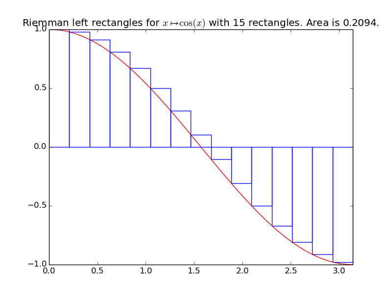
integrals.riemann_left(f, xmin, xmax, n=1000)

Compute an approximation of the integral of the function f from \(x_{\min}\) to \(x_{\max}\), by using n Riemann left rectangles:

\[\displaystyle \int_{x=x_{\min}}^{x=x_{\max}} f(x) \mathrm{d}x \approx \sum_{i=0}^{n-1} \left( h \times f(x_{\min} + i h) \right).\]

For this method and the next ones, we take \(n\) points, and \(h\) is defined as \(h = \frac{x_{\max} - x_{\min}}{n}\), the horizontal size of the rectangles (or trapeziums).

Example for riemann_left():

A first example on a trignometric function with nice bounds:

>>> exact_int = math.sin(math.pi) - math.sin(0)
>>> exact_int  
1.22...e-16
>>> round(exact_int, 0)
0.0
>>> left_int = riemann_left(math.cos, 0, math.pi, n=15); left_int  
0.2094...
>>> round(100*abs(exact_int - left_int), 0)  # Relative % error of 21%, VERY BAD!
21.0

integrals.plot_riemann_left(f, xmin, xmax, namef='$f(x)$', n=10, figname=None)

Plot the function f from \(x_{\min}\) to \(x_{\max}\), and n Riemann left rectangles.

Example:

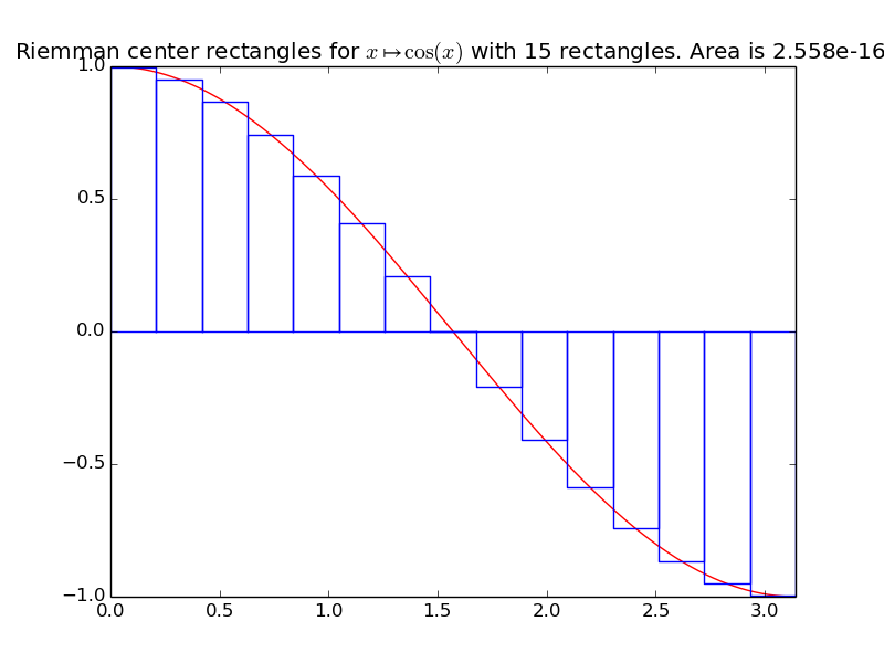
integrals.riemann_center(f, xmin, xmax, n=1000)

Compute an approximation of the integral of the function f from \(x_{\min}\) to \(x_{\max}\), by using n Riemann center rectangles:

\[\displaystyle \int_{x=x_{\min}}^{x=x_{\max}} f(x) \mathrm{d}x \approx \sum_{i=0}^{n-1} \left( h \times f(x_{\min} + (i + \frac{1}{2}) * h) \right).\]

Example for riemann_center():

A first example on a trignometric function with nice bounds:

>>> exact_int = math.sin(math.pi) - math.sin(0); round(exact_int, 0)
0.0
>>> center_int = riemann_center(math.cos, 0, math.pi, n=15); center_int  
2.918...e-16
>>> round(100*abs(exact_int - center_int), 0)  # % Error
0.0

integrals.plot_riemann_center(f, xmin, xmax, namef='$f(x)$', n=10, figname=None)

Plot the function f from \(x_{\min}\) to \(x_{\max}\), and n Riemann left rectangles.

Example:

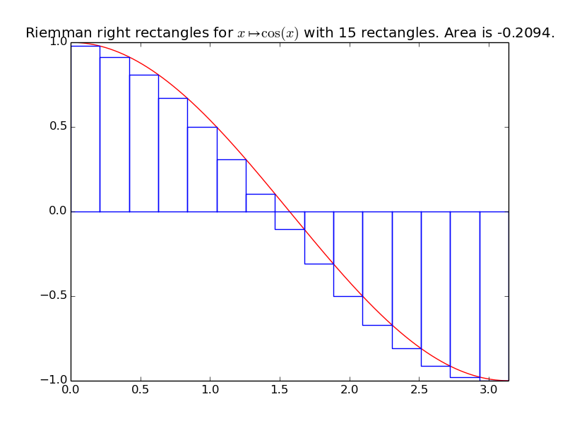
integrals.riemann_right(f, xmin, xmax, n=1000)

Compute an approximation of the integral of the function f from \(x_{\min}\) to \(x_{\max}\), by using n Riemann right rectangles:

\[\displaystyle \int_{x=x_{\min}}^{x=x_{\max}} f(x) \mathrm{d}x \approx \sum_{i=1}^{n} \left( h \times f(x_{\min} + i h) \right).\]

Example for riemann_right():

A first example on a trignometric function with nice bounds:

>>> exact_int = math.sin(math.pi) - math.sin(0); round(exact_int, 0)
0.0
>>> right_int = riemann_right(math.cos, 0, math.pi, n=15); right_int  
-0.2094...
>>> round(100*abs(exact_int - right_int), 0)  # % Error
21.0

The more rectangles we compute, the more accurate the approximation will be:

>>> right_int = riemann_right(math.cos, 0, math.pi, n=2000); right_int  
-0.00157...
>>> 100*abs(exact_int - right_int)  # Error is less than 0.15 %  
0.15...
>>> round(100*abs(exact_int - right_int), 0)  # % Error
0.0

integrals.plot_riemann_right(f, xmin, xmax, namef='$f(x)$', n=10, figname=None)

Plot the function f from \(x_{\min}\) to \(x_{\max}\), and n Riemann left rectangles.

Example:

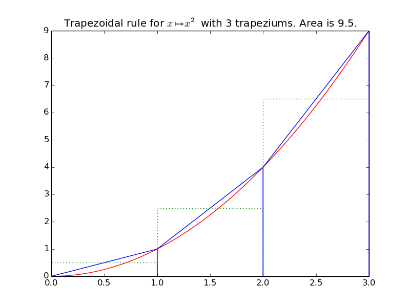
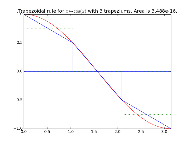
integrals.trapez(f, xmin, xmax, n=1000)

Compute an approximation of the integral of the function f from \(x_{\min}\) to \(x_{\max}\), by using n trapeziums:

\[\displaystyle \int_{x=x_{\min}}^{x=x_{\max}} f(x) \mathrm{d}x \approx \sum_{i=0}^{n-1} \left( h \times \frac{f(x_{\min} + i h) + f(x_{\min} + (i+1) * h)}{2} \right).\]

Example for trapez():

A first example on a trignometric function with nice bounds:

>>> exact_int = math.sin(math.pi) - math.sin(0); round(exact_int, 0)
0.0
>>> trapez_int = trapez(math.cos, 0, math.pi, n=15); trapez_int  
2.281...e-16
>>> round(100*abs(exact_int - trapez_int), 0)  # % Error
0.0

integrals.plot_trapez(f, xmin, xmax, namef='$f(x)$', n=10, figname=None)

Plot the function f from \(x_{\min}\) to \(x_{\max}\), and n trapeziums.

Example:

integrals.yminmax(f, xmin, xmax, n=10000, threshold=0.005)

Experimental guess of the values \(y_{\min}, y_{\max}\) for f, by randomly picking \(n\) points.

• threshold is here to increase a little bit the size of the window, to be cautious. Default is 0.5%.
• Note: there are more efficient and trustworthy methods, but this one is a simple one.

Warning

Not sure if the threshold is mathematically a good idea...

Example for yminmax():

Just to try, on an easy function (degree 2 polynomial):

>>> random.seed(1)  # same values all the time
>>> ymin_exact, ymax_exact = -0.25, 12
>>> ymin, ymax = yminmax(lambda x: x**2 + x, -2, 3, 200)
>>> ymin, ymax  
(-0.251..., 12.059...)
>>> 100 * abs(ymin - ymin_exact) / abs(ymin_exact)  # Relative % error < 0.5%  
0.480...
>>> 100 * abs(ymax - ymax_exact) / abs(ymax_exact)  # Relative % error < 0.5%  
0.499...

integrals.montecarlo(f, xmin, xmax, n=10000, ymin=None, ymax=None)

Compute an approximation of the integral of \(f(x)\) for \(x\) from \(x_{\min}\) to \(x_{\max}\).

• Each point \((x, y)\) is taken in the rectangle \([x_{\min}, x_{\max}] \times [y_{\min}, y_{\max}]\).
• \(n\) is the number of random points to pick (it should be big, like 1000 at least).
• What is returned is \(\text{area} \approx (\text{Area rectangle}) \times (\text{Estimated ratio})\):

\[\text{area} \approx (x_{\max} - x_{\min}) \times (y_{\max} - y_{\min}) \times \frac{\text{Nb points below the curve}}{\text{Nb points}}.\]

Warning

The values \(y_{\min}\) and \(y_{\max}\) should satisfy \(y_{\min} \leq \mathrm{\min}(\{ f(x): x_{\min} \leq x \leq x_{\max} \})\) and \(\mathrm{\max}(\{ f(x): x_{\min} \leq x \leq x_{\max} \}) \leq y_{\max}\).

Example 1 for montecarlo():

For example, we are interested in \(\int_1^6 x \mathrm{d} x = \frac{6^2}{2} - \frac{1^6}{2} = 17.5\).

>>> random.seed(1)  # same values all the time
>>> xmin, xmax = 1, 6
>>> f = lambda x: x  # simple example
>>> intf = (xmax**2 / 2.0) - (xmin**2 / 2.0); intf
17.5
>>> ymin, ymax = xmin, xmax

Let us start by taking 100 points:

>>> n = 100
>>> intf_apporx = montecarlo(f, xmin, xmax, n, ymin, ymax); intf_apporx
18.0
>>> 100 * abs(intf - intf_apporx) / abs(intf)  # Relative % error, 2.8%  
2.857...

The more points we take, the better the approximation will be:

>>> n = 100000
>>> intf_apporx = montecarlo(f, xmin, xmax, n, ymin, ymax); intf_apporx  
17.444...
>>> 100 * abs(intf - intf_apporx) / abs(intf)  # Relative % error, 0.32%  
0.318...

Example 2 for montecarlo():

We can also let the function compute ymin and ymax by itself:

>>> n = 100000
>>> intf_apporx = montecarlo(f, xmin, xmax, n); intf_apporx  
17.485...
>>> 100 * abs(intf - intf_apporx) / abs(intf)  # Relative % error, 0.08% is really good!  
0.0844...

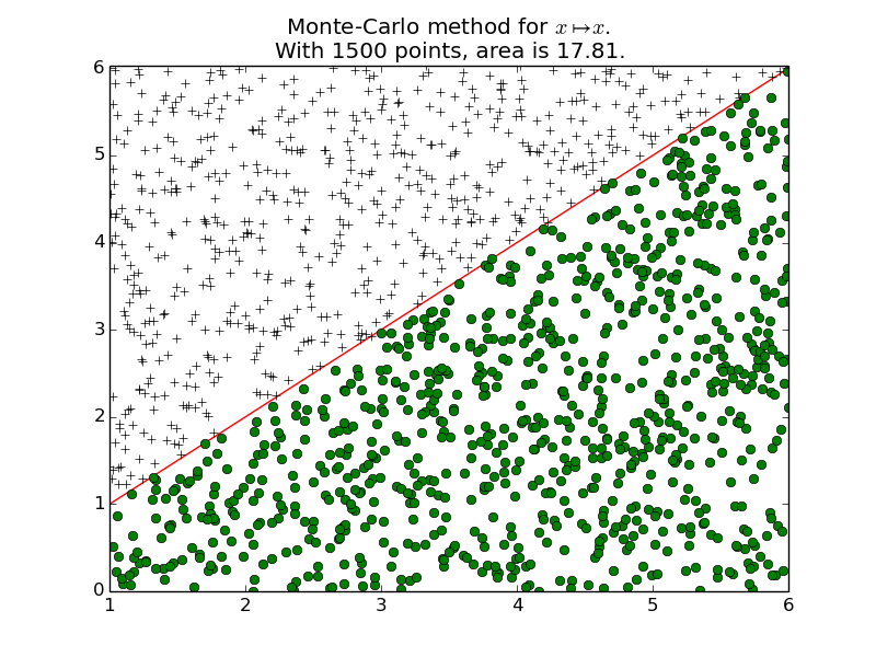
integrals.plot_montecarlo(f, xmin, xmax, n=1000, ymin=None, ymax=None, namef='$f(x)$', figname=None)

Plot the function f from \(x_{\min}\) to \(x_{\max}\), and \(n\) random points.

• Each point \((x, y)\) is taken in the rectangle \([x_{\min}, x_{\max}] \times [y_{\min}, y_{\max}]\).
• Warning: \(y_{\min}\) and \(y_{\max}\) should satisfy \(y_{\min} \leq \mathrm{\min}(\{ f(x): x_{\min} \leq x \leq x_{\max} \})\) and \(\mathrm{\max}(\{ f(x): x_{\min} \leq x \leq x_{\max} \}) \leq y_{\max}\).

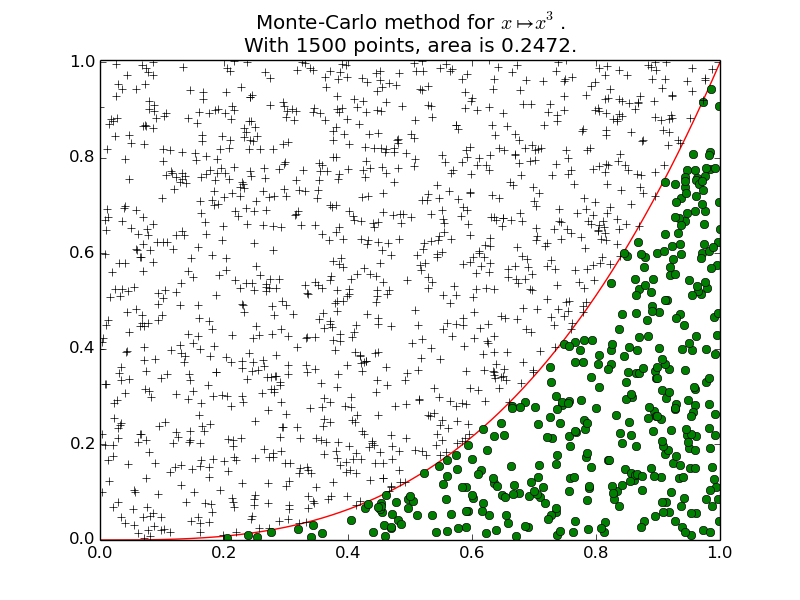
Example 1 for plot_montecarlo():

A first example: \(\int_0^1 x^3 \mathrm{d}x = \frac{1}{4} = 0.25\).

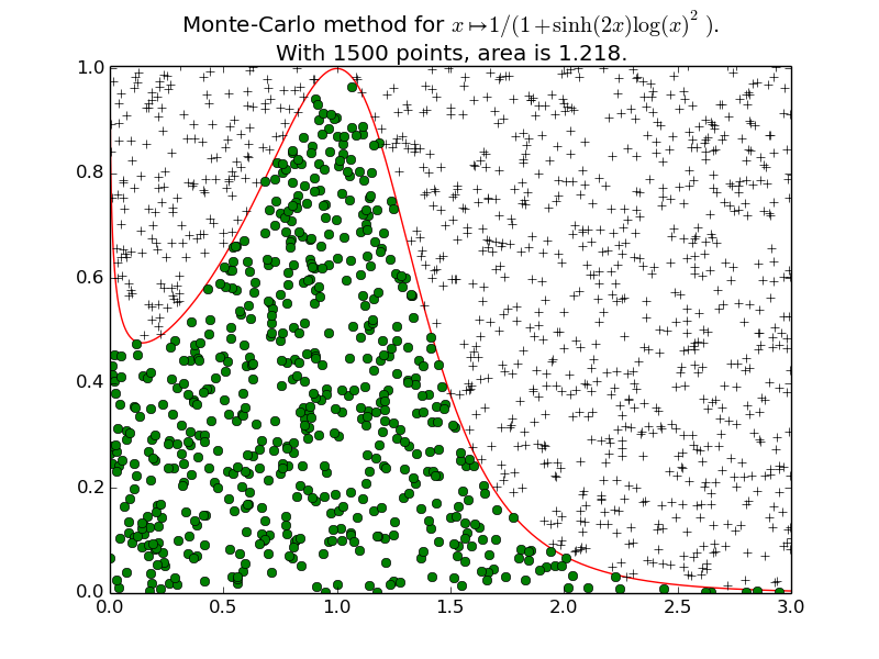
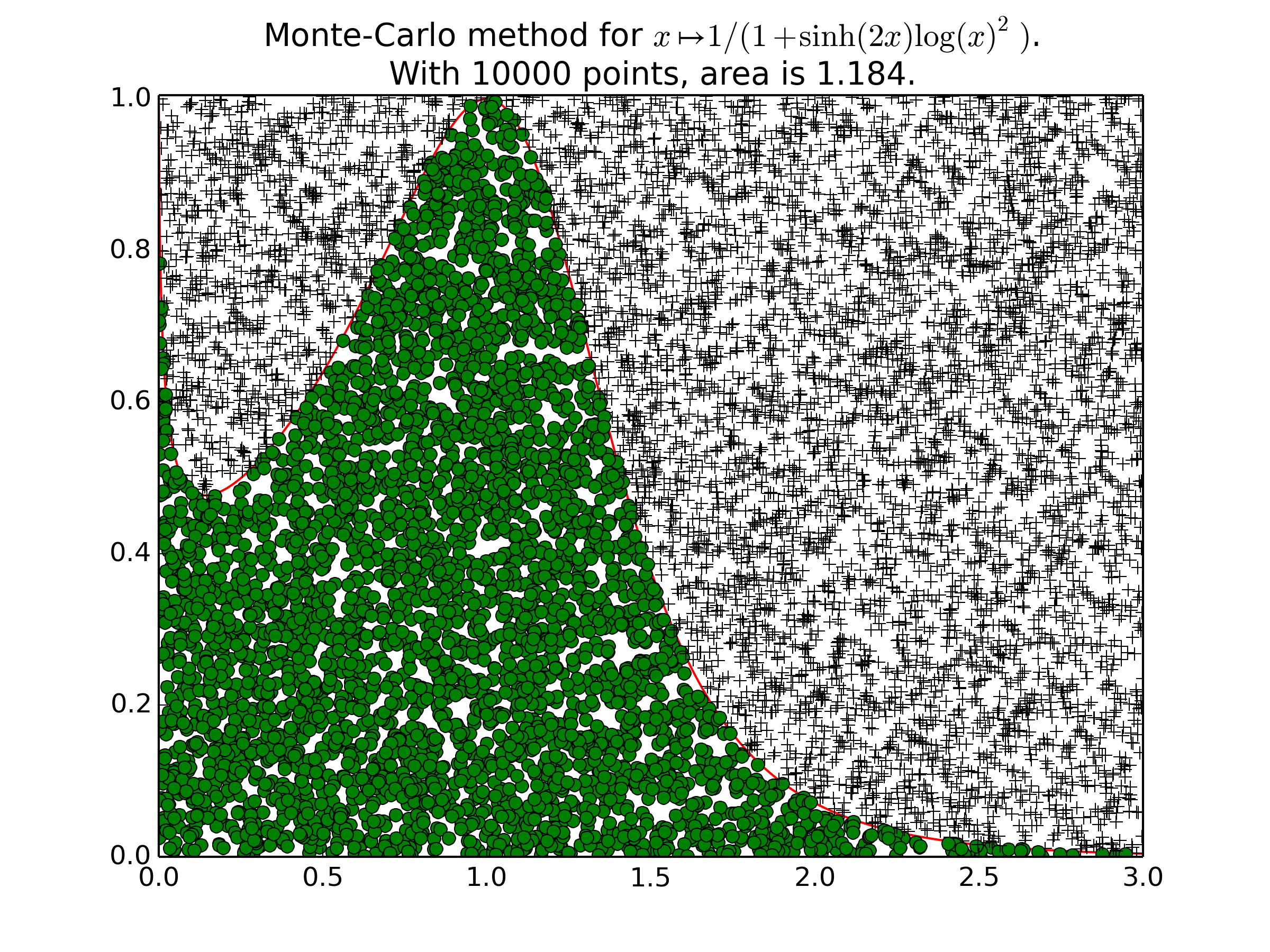
Example 2 for plot_montecarlo():

Another example on a less usual function (\(f(x) = \frac{1}{1+\mathrm{sinh}(2x) \log(x)^2}\)), with \(1500\) points, and then \(10000\) points.

integrals.simpson(f, xmin, xmax, n=1000)

Compute an approximation of the integral of the function f from \(x_{\min}\) to \(x_{\max}\), by using composite Simpson’s rule.

\[\displaystyle \int_{x=x_{\min}}^{x=x_{\max}} f(x) \mathrm{d}x \approx \tfrac{h}{3} \bigg(f(x_0)+2\sum_{j=1}^{n/2-1}f(x_{2j})+ 4\sum_{j=1}^{n/2}f(x_{2j-1})+f(x_n)\bigg),\]

where \(x_j = x_{\min} + j h\) for \(j=0, 1, \dots, n-1, n\) and \(h = \frac{x_{\max} - x_{\min}}{n}\).

Example 1 for simpson():

A first example on a trignometric function with nice bounds:

>>> exact_int = math.sin(math.pi) - math.sin(0); round(exact_int, 0)
0.0
>>> simpson_int = simpson(math.cos, 0, math.pi, n=10)
>>> simpson_int; abs(round(simpson_int, 0))  
9.300...e-17
0.0
>>> round(100*abs(exact_int - simpson_int), 0)  # % Error
0.0

• References are Simpson’s Rule (on MathWorld) and Simpson’s Rule (on Wikipedia),
• The function \(f\) is evaluated \(n\) number of times,
• This method is exact upto the order 3 (ie. the integral of polynomials of degree \(\leq 3\) are computed exactly):

>>> f = lambda x: (x**2) + (7*x) + (4)
>>> F = lambda x: ((x**3)/3.0) + ((7 * x**2)/2.0) + (4*x)
>>> a, b = -1, 12
>>> exact_int2 = F(b) - F(a); round(exact_int2, 0)
1129.0
>>> simpson_int2 = simpson(f, a, b, n=2)
>>> simpson_int2; abs(round(simpson_int2, 0))
1128.8333333333333
1129.0
>>> round(100*abs(exact_int2 - simpson_int2), 0)  # % Error
0.0

Example 2 for simpson():

One more example (coming from Wikipédia), to show that this method is exact upto the order 3:

>>> round(simpson(lambda x:x**3, 0.0, 10.0, 2), 7)
2500.0
>>> round(simpson(lambda x:x**3, 0.0, 10.0, 10000), 7)
2500.0

But not from the order 4:

>>> round(simpson(lambda x:x**4, 0.0, 10.0, 2), 7)
20833.3333333
>>> round(simpson(lambda x:x**4, 0.0, 10.0, 100000), 7)
20000.0

Example 3 for simpson():

A random example: \(\displaystyle \int_{1993}^{2015} \left( \frac{1+12x}{1+\cos^2(x)} \right) \mathrm{d}x\):

>>> f = lambda x: (12*x+1) / (1+math.cos(x)**2)
>>> a, b = 1993, 2015
>>> simpson(f, a, b, n=2)  
345561.243...
>>> simpson(f, a, b, n=8)  
374179.344...
>>> simpson(f, a, b, n=100)  
374133.138...

The value seems to be 374133.2, as confirmed by Wolfram|Alpha. The same example will also be used for other function, see below.

integrals.boole(f, xmin, xmax, n=1000)

Compute an approximation of the integral of the function f from \(x_{\min}\) to \(x_{\max}\), by using composite Boole’s rule.

\[\displaystyle \int_{x=x_{\min}}^{x=x_{\max}} f(x) \mathrm{d}x \approx \tfrac{2h}{45} \sum_{i=0}^{n}\bigg(7f(x_{i}) + 32f(x_{i+1}) + 12f(x_{i+2}) + 32f(x_{i+3}) + 7f(x_{i+4})\bigg),\]

where \(x_i = x_{\min} + i h\) for \(i=0, 1, \dots, 4n-1, 4n\) and \(h = \frac{x_{\max} - x_{\min}}{4*n}\).

Example 1 for boole():

A first example on a trignometric function with nice bounds:

>>> exact_int = math.sin(math.pi) - math.sin(0); round(exact_int, 0)
0.0
>>> boole_int = boole(math.cos, 0, math.pi, n=10)
>>> boole_int; abs(round(boole_int, 0))  
1.612...e-16
0.0
>>> round(100*abs(exact_int - boole_int), 0)  # % Error
0.0

• Reference is Boole’s Rule (on MathWorld), and Boole’s Rule (on Wikipedia),
• The function \(f\) is evaluated \(4 n\) number of times,
• This method is exact upto the order 4 (ie. the integral of polynomials of degree \(\leq 4\) are computed exactly).

Example 2 for boole():

A second easy example on a degree 3 polynomial:

>>> f = lambda x: (x**3) + (x**2) + (7*x) + 4
>>> F = lambda x: (x**4)/4.0 + (x**3)/3.0 + (7 * x**2)/2.0 + (4*x)
>>> a, b = -4, 6
>>> exact_int2 = F(b) - F(a); round(exact_int2, 0)
463.0
>>> boole_int2 = boole(f, a, b, n=10)  # n = 10 is good enough!
>>> boole_int2; abs(round(boole_int2, 6))  # Weird!
463.33333333333337
463.333333
>>> round(100*abs(exact_int2 - boole_int2), 0)  # % Error
0.0

Example 3 for boole():

On the same harder example:

>>> f = lambda x: (12*x+1)/(1+math.cos(x)**2)
>>> a, b = 1993, 2015
>>> boole(f, a, b, n=1)  
373463.255...
>>> boole(f, a, b, n=2)  
374343.342...
>>> boole(f, a, b, n=100)  # Really close to the exact value.  
374133.193...

integrals.romberg_rec(f, xmin, xmax, n=8, m=None)

Compute the \(R(n, m)\) value recursively, to approximate \(\int_{x_{\min}}^{x_{\max}} f(x) \mathrm{d}x\).

• The integrand \(f\) must be of class \(\mathcal{C}^{2n+2}\) for the method to be correct.
• Time complexity is \(O(2^{n m})\) and memory complexity is also \(O(2^{n m})\).
• Warning: the time complexity is increasing very quickly with respect to \(n\) here, be cautious.

Example for romberg_rec():

On the same hard example as above:

>>> f = lambda x: (12*x+1)/(1+math.cos(x)**2)
>>> a, b = 1993, 2015
>>> romberg_rec(f, a, b, n=0)  # really not accurate!  
477173.613...
>>> romberg_rec(f, a, b, n=1)  # alreay pretty good!  
345561.243...
>>> romberg_rec(f, a, b, n=2)  
373463.255...
>>> romberg_rec(f, a, b, n=3)  
374357.311...
>>> romberg_rec(f, a, b, n=8)  # Almost the exact value.  
374133.192...

We should not go further (\(4^n\) is increasing quickly!). With a bigger order, this recursive implementation will fail (because of the tail recursion limit, about 1000 in Python 3)!

integrals.romberg(f, xmin, xmax, n=8, m=None, verb=False)

(Inductively) compute the \(R(n, m)\) value by using dynamic programming, to approximate \(\int_{x_{\min}}^{x_{\max}} f(x) \mathrm{d}x\). This solution is way more efficient that the recursive one!

• The integrand \(f\) must be of class \(\mathcal{C}^{2n+2}\) for the method to be correct.
• Note: a memoization trick is too hard to set-up here, as this value \(R(n, m)\)) depends on f, a and b.
• Time complexity is \(O(n m)\) and memory complexity is also \(O(n m)\) (using a dictionary to store all the value \(R(i, j)\) for all the indeces \(0 \leq i \leq n, 0 \leq j \leq m, j \leq i\)).

Example 1 for romberg():

Let us start with a first example from the Wikipedia page for Romberg’s method: \(\int_{0}^{1} \exp(-x^2) \mathrm{d}x \approx 0.842700792949715\):

>>> f = lambda x: (2.0 / math.sqrt(math.pi)) * math.exp(-x**2)
>>> erf1 = romberg(f, 0, 1, 5, 5); erf1  
0.84270...
>>> exact_erf1 = 0.842700792949715  # From Wikipedia
>>> 100 * abs(erf1 - exact_erf1)  # Absolute % error, 2e-11 is almost perfect!  
2.070...e-11

We can check that \(\int_{0}^{\pi} \sin(x) \mathrm{d}x = 2\), with n = m = 5:

>>> area = romberg(math.sin, 0, math.pi, 5, 5); area
2.0000000000013207
>>> 100 * abs(area - 2.0)  # Absolute % error, 1e-10 is already very good!  
1.320...e-10

We check that romberg() is also working for functions that are not always positive (alternating between being positive and being negative): \(\int_{0}^{1001 \pi} \sin(x) \mathrm{d}x = \int_{1000 \pi}^{1001 \pi} \sin(x) \mathrm{d}x = \int_{0}^{\pi} \sin(x) \mathrm{d}x = 2\):

>>> area2 = romberg(math.sin, 0, 1001*math.pi, 5, 5); area2  
-148.929...
>>> 100 * abs(area2 - 2.0)  # Really bad here!  
15092.968...
>>> area3 = romberg(math.sin, 0, 1001*math.pi, 15, 15); area3  
1.999...
>>> 100 * abs(area3 - 2.0)  # Should be better: yes indeed, an absolute error of 3e-09 % is quite good!  
3.145...e-09

Example 2 for romberg():

Now, I would like to consider more examples, they will all be computed with n = m = 5:

>>> n = m = 5
>>> a = 0; b = 1

First, we can compute an approximation of \(\frac{\pi}{4}\) by integrating the function \(f_1(x) = \sqrt{1-x^2}\) on \([0, 1]\):

>>> f1 = lambda x: (1-x**2)**0.5
>>> int_f1 = romberg(f1, a, b, n, m); int_f1  
0.784...
>>> 100 * abs(int_f1 - math.pi / 4.0)  # 0.05%, that's really good!  
0.053...

For \(f_2(x) = x^2\), \(\int_{0}^{1} f_2(x) \mathrm{d}x = \frac{1}{3}\):

>>> f2 = lambda x: x**2
>>> int_f2 = romberg(f2, a, b, n, m); int_f2
0.3333333333333333
>>> 100 * abs(int_f2 - 1.0/3.0)
0.0

For \(f_3(x) = \sin(x)\), \(\int_{0}^{\pi} f_3(x) \mathrm{d}x = 2\):

>>> f3 = math.sin; b = math.pi
>>> int_f3 = romberg(f3, a, b, n, m); int_f3
2.0000000000013207
>>> 100 * abs(int_f3 - 2.0)  # 10e-10 % error, that's almost perfect!  
1.320...e-10

Example 3 for romberg():

For \(f_4(x) = \exp(x)\), it is easy to compute any integrals: \(\int_{-4}^{19} f_4(x) \mathrm{d}x = \int_{-4}^{19} \exp(x) \mathrm{d}x = \exp(19) - \exp(-4)\):

>>> f4 = math.exp
>>> n, m = 5, 5
>>> a, b = -4, 19
>>> int_f4 = romberg(f4, a, b, n, m); int_f4  
178495315.533...
>>> exact_f4 =  f4(b) - f4(a); exact_f4  
178482300.944...
>>> 100 * abs(int_f4 - exact_f4)  # Not so good result! n=m=5 is not enough  
1301458.822...

As we can see, the result is not satisfactory with n = m = 5 and for a function \(f\) that can take “big” and “small” values on the integration interval (\([a, b]\)).

Now what happens if we increase the value of n (and keep m = n)?

>>> n, m = 10, 10   # More points!
>>> int_f4_2 = romberg(f4, a, b, n, m); int_f4_2  
178482300.944...
>>> exact_f4_2 =  f4(b) - f4(a)
>>> 100 * abs(int_f4_2 - exact_f4_2)  # A smaller error!  
5.960...e-06

Another example on a “big” integral and a “big” interval (the numerical value of the integral is bigger):

>>> a, b = -1000, 20; n, m = 10, 10   # More points!
>>> int_f4_3 = romberg(f4, a, b, n, m); int_f4_3  
485483299.278...
>>> exact_f4_3 =  f4(b) - f4(a); exact_f4_3  
485165195.409...
>>> 100 * abs(int_f4_3 - exact_f4_3)  # It is not accurate for big intervals  
31810386.832...

Let compare with this not-so-accurate result (obtained with n = m = 10), with the one given with n = m = 20:

>>> a, b = -1000, 20; n, m = 20, 20   # More points! n=m=20 is really big!
>>> int_f4_4 = romberg(f4, a, b, n, m); int_f4_4  
485165195.409...
>>> 100 * abs(int_f4_4 - exact_f4_3)
0.0

Example 4 for romberg():

On the same example as above (for simpson() and boole(), to compare the two implementations of the Romberg’s method:

>>> f = lambda x: (12*x+1)/(1+math.cos(x)**2)
>>> a, b = 1993, 2015
>>> romberg(f, a, b, n=0)  # really not accurate!  
477173.613...
>>> romberg(f, a, b, n=1)  
345561.243...
>>> romberg(f, a, b, n=2)  
373463.255...
>>> romberg(f, a, b, n=3)  
374357.311...
>>> romberg(f, a, b, n=5)  
374134.549...

At one point, increasing the value of \(n\) does not change the result anymore (due to the limited precision of float computations):

>>> romberg(f, a, b, n=8)  # Almost the exact value.  
374133.192...
>>> romberg(f, a, b, n=10)  # More precise!  
374133.193...
>>> romberg(f, a, b, n=14)  # Again more precise!  
374133.193...
>>> romberg(f, a, b, n=20)  # Exact value!  
374133.193...

integrals.xw_gauss_legendre(n)

Experimental caching of the xi, wi values returned by p_roots, to be more efficient for higher order Gaussian quadrature.

• Higher order quadratures call several times the function scipy.special.orthogonal.p_roots() with the same parameter n, so it is easy to be more efficient, by caching the values xi, wi generated by this call.

integrals.gaussian_quad(f, xmin, xmax, n=10)

Integrates between \(x_{\min}\) and \(x_{\max}\), using Gaussian quadrature.

• The weigts and roots of the Gauss-Legendre polynomials are computed by SciPy (scipy.special.orthogonal.p_roots()).
• Complexity of my part is \(O(n)\), but I don’t know how efficient is the p_roots function.
• I added a cache layer to the p_roots function (see xw_gauss_legendre()).

Example for gaussian_quad():

Same example as previously:

>>> f = lambda x: (12*x+1)/(1+math.cos(x)**2)
>>> a, b = 1993, 2015
>>> gaussian_quad(f, a, b, n=1)  
279755.057...
>>> gaussian_quad(f, a, b, n=3)  
343420.473...
>>> gaussian_quad(f, a, b, n=100)  # Quite accurate result, see above.  
374133.206...

integrals.dbl_quad(f, a, b, g, h, n=10)

Double integrates \(f(x, y)\), when \(y\) is moving between \(g(x)\) and \(h(x)\) and when \(x\) is moving between \(a\) and \(b\), by using two interlaced Gaussian quadratures.

• Based on Fubini’s Theorem, for integrals of the forms \(\displaystyle \iint_D f(x, y) \mathrm{d}x \mathrm{d}y = \int_{x = a}^{x = b}\left(\int_{y = g(x)}^{y = h(x)} f(x) \mathrm{d}y \right) \mathrm{d}x.\)

Example 1 for dbl_quad():

For example, \(\int_{x = 0}^{x = 1}\bigg(\int_{y = 0}^{y = 1} \left( x^2 + y^2 \right) \mathrm{d}y \bigg) \mathrm{d}x = 2 \int_{0}^{1} x^2 \mathrm{d}x = 2 \frac{1^3}{3} = 2/3\):

>>> f = lambda x, y:  x**2 + y**2
>>> a, b = 0, 1
>>> g = lambda x: a
>>> h = lambda x: b
>>> dbl_quad(f, a, b, g, h, n=1)
0.5
>>> dbl_quad(f, a, b, g, h, n=2)  # exact from n=2 points
0.66666666666666674
>>> dbl_quad(f, a, b, g, h, n=40)  # more points do not bring more digits
0.66666666666666574

Example 2 for dbl_quad():

A second example could be: \(\int_{x = 0}^{x = \pi/2}\bigg(\int_{y = 0}^{y = \pi/2} \left( \cos(x) y^8 \right) \mathrm{d}y \bigg) \mathrm{d}x\).

>>> f = lambda x, y:  math.cos(x) * y**8
>>> a, b = 0, math.pi/2.0
>>> g = lambda x: a
>>> h = lambda x: b

This integral can be computed mathematically \(\int_{x = 0}^{x = \pi/2}\bigg(\int_{y = 0}^{y = \pi/2} \left( \cos(x) y^8 \right) \mathrm{d}y \bigg) \mathrm{d}x = \frac{(\pi/2)^9}{9} \int_{0}^{\pi/2} \cos(x) \mathrm{d}x = \frac{(\pi/2)^9}{9} \approx 6.468988\)

>>> int2d_exact = (b**9) / 9.0; int2d_exact  
6.4689...

Let see how efficient is the double Gaussian quadrature method:

>>> dbl_quad(f, a, b, g, h, n=1)  
0.2526...
>>> dbl_quad(f, a, b, g, h, n=2)  # still not very precise for n=2 points  
4.3509...

With \(n = 40\), we have \(n^2 = 40^2 = 1600\) points:

>>> int2d_approx = dbl_quad(f, a, b, g, h, n=40); int2d_approx  # 13 first digits are perfect  
6.4689...
>>> 100 * abs(int2d_exact - int2d_approx) / int2d_exact  # Relative % error, 1e-12 is VERY SMALL  
6.59...e-13
>>> 100 * abs(int2d_exact - int2d_approx)  # Absolute % error, 1e-12 is really good!  
4.263...e-12

We see again that all these methods are limited to a precision of 12 to 14 digits, because we use Python float numbers (IEEE-754 floating point arithmetic).

Example 3 for dbl_quad():

3 examples are given here, with moving bounds: \(g(x)\) or \(h(x)\) are really depending on \(x\).

The first one is \(\displaystyle \iint_{(x, y) \in D_1} \cos(y^2) \;\; \mathrm{d}(x,y) = \int_0^1 \int_{x}^{1} \cos(y^2) \;\; \mathrm{d}y \mathrm{d}x = \frac{\sin(1)}{2} \approx 0.4207354924039\):

>>> a1, b1 = 0, 1
>>> g1 = lambda x: x; h1 = lambda x: 1
>>> f1 = lambda x, y: math.cos(y**2)
>>> exact_dbl_int1 = math.sin(1.0) / 2.0; exact_dbl_int1  
0.4207...
>>> dbl_int1 = dbl_quad(f1, a1, b1, g1, h1, n=4)
>>> dbl_int1  
0.4207...
>>> 100 * abs(dbl_int1 - exact_dbl_int1)  # Not perfect yet, n is too small  
3.933...e-05
>>> dbl_int1 = dbl_quad(f1, a1, b1, g1, h1, n=100)
>>> dbl_int1  
0.4207...
>>> 100 * abs(dbl_int1 - exact_dbl_int1)  # Almost perfect computation (13 digits are correct)  
0.0

Note

Solved with SymPy integrals module:

This program on bitbucket.org/lbesson/python-demos (written in January 2015), uses SymPy to symbolically compute this double integral.

The second one is computing the area between the curves \(y = x^2\) and \(y = \sqrt{x}\), for \(x \in [0, 1]\): \(\displaystyle \text{Area}(D_2) = \iint_{(x, y) \in D_2} 1 \;\; \mathrm{d}(x,y) = \int_0^1 \int_{x^2}^{\sqrt{x}} 1 \;\; \mathrm{d}y \mathrm{d}x = \frac{2}{3} - \frac{1}{3} = \frac{1}{3}\):

>>> a2, b2 = 0, 1
>>> g2 = lambda x: x**2; h2 = lambda x: x**0.5
>>> f2 = lambda x, y: 1
>>> exact_dbl_int2 = 1.0 / 3.0
>>> dbl_int2 = dbl_quad(f2, a2, b2, g2, h2, n=100)
>>> dbl_int2  
0.3333...
>>> 100 * abs(dbl_int2 - exact_dbl_int2)  # 0.0001% is very good!  
1.01432...e-05

The last one is \(\displaystyle \iint_{(x, y) \in D_3} \frac{\sin(y)}{y} \;\; \mathrm{d}(x,y) = \int_0^1 \int_{x}^{1} \frac{\sin(y)}{y} \;\; \mathrm{d}y \mathrm{d}x = 1 - \cos(1) \approx 0.45969769413186\):

>>> a3, b3 = 0, 1
>>> g3 = lambda x: x; h3 = lambda x: 1
>>> f3 = lambda x, y: math.sin(y) / y
>>> exact_dbl_int3 = 1 - math.cos(1.0); exact_dbl_int3
0.45969769413186023
>>> dbl_int3 = dbl_quad(f3, a3, b3, g3, h3, n=100)
>>> dbl_int3
0.4596976941318604
>>> 100 * abs(dbl_int3 - exact_dbl_int3)  # Almost perfect computation (14 digits are correct)  
1.665...e-14

Note

All these examples are coming from the MA102 quiz given on January the 29th, 2015.

integrals.nd_quad(f, Xmin, Xmax, n=10)

k-dimensional integral of \(f(\overrightarrow{x})\), on a hypercube (k-dimensional square) \(D = [\text{Xmin}_1, \text{Xmax}_1] \times \dots \times [\text{Xmin}_k, \text{Xmax}_k]\), by using k interlaced Gaussian quadratures.

• Based on the generalized Fubini’s Theorem, for integrals of the forms \(\displaystyle \int_D f(\overrightarrow{x}) \mathrm{d}\overrightarrow{x} = \int_{x_1=\text{Xmin}_1}^{x_1=\text{Xmax}_1} \int_{x_2=\text{Xmin}_2}^{x_2=\text{Xmax}_2} \dots \int_{x_k=\text{Xmin}_k}^{x_k=\text{Xmax}_k} f(x_1, x_2, \dots, x_k) \mathrm{d}x_k \dots \mathrm{d}x_2 \mathrm{d}x_1\).
• The function f has to accept an iterable of size k (list, tuple, numpy array?).
• Right now, we are taking about \(O(n^k)\) points, so do not take a too big value for n.
• See this trick which explains how to integrate a function on a more complicated domain. The basic concept is to include the knowledge of the domain (inequalities, equalities) in the function f itself.

Example 1 for nd_quad():

First example, volume of a 3D sphere:

For example, we can compute the volume of a 3D sphere of radius R: \(V_R = \frac{4}{3} \pi R^3\), by integrating the function \(f : X \mapsto 1\) on the cube \([-R, R]^3\).

>>> R = 1
>>> f = lambda X: 1

For \(R = 1\), \(V_R = V_1 \approx 4.18879\):

>>> V_3 = (4.0/3.0) * math.pi * (R**3); V_3  
4.18879...

The trick is to multiply \(f(X)\) by 1 if \(X\) is inside the sphere, or by 0 otherwise:

>>> isInside = lambda X: 1 if (sum(x**2 for x in X) <= R**2) else 0
>>> F = lambda X: f(X) * isInside(X)

Then we integrate on \([0, R]^3\) to get \(1/8\) times the volume (remember that the smaller the integration domain, the more efficient the method will be):

>>> Xmin = [0, 0, 0]; Xmax = [R, R, R]
>>> (2**3) * nd_quad(F, Xmin, Xmax, n=2)
4.0
>>> (2**3) * nd_quad(F, Xmin, Xmax, n=4)
4.0
>>> (2**3) * nd_quad(F, Xmin, Xmax, n=8)
4.3182389695603307

The more points we consider, the better the approximation will be (as usual):

>>> V_approx10 = (2**3) * nd_quad(F, Xmin, Xmax, n=10); V_approx10  
4.12358...
>>> 100 * abs(V_3 - V_approx10) / abs(V_3)  # Relative % error, 1.5% is OK  
1.55...
>>> V_approx40 = (2**3) * nd_quad(F, Xmin, Xmax, n=40); V_approx40  
4.18170...
>>> 100 * abs(V_3 - V_approx40) / abs(V_3)  # Relative % error, 0.16% is good  
0.16...

Example 2 for nd_quad():

Second example, volume of a n-ball:

We can also try to compute the volume of a higher dimensional ball: \(\displaystyle V_{k, R} = \frac{\pi^{k/2}}{\Gamma(k/2 + 1)} R^k\).

>>> from math import gamma, pi
>>> V = lambda k, R: (pi**(k/2.0))/(gamma( 1 + k/2.0 )) * (R**k)

A ball of radius \(R = 1\) in dimension \(k = 5\) will have a 5-dim volume of \(\frac{8\pi^2}{15} R^{5} \approx 5.263789013914325\):

>>> k = 5; R = 1
>>> V_5 = V(k, R); V_5  # Exact value!  
5.26378...

Similarly, the integration domain can be \([0, 1] \times \dots \times [0, 1]\).

>>> Xmin = [0]*k; Xmax = [1]*k
>>> isInside = lambda X: 1 if (sum(x**2 for x in X) <= R**2) else 0
>>> F = lambda X: 1.0 * isInside(X)
>>> V_approx5_3 = (2**k) * nd_quad(F, Xmin, Xmax, n=3)  # 3**5 = 243 points, so really not accurate
>>> V_approx5_3  
4.2634...
>>> 100 * abs(V_5 - V_approx5_3) / abs(V_5)  # n=3 gives an error of 19%, that's not too bad!  
19.0049...

Exactly as before, we can try to take more points:

>>> V_approx5_10 = (2**k) * nd_quad(F, Xmin, Xmax, n=10)  # 10**5 = 10000 points!
>>> V_approx5_10  
5.25263...
>>> 100 * abs(V_5 - V_approx5_10) / abs(V_5)  # Pretty good!  
0.211...
>>> V_approx5_15 = (2**k) * nd_quad(F, Xmin, Xmax, n=15)  # 15**5 = 759375 points!
>>> V_approx5_15  
5.24665...
>>> 100 * abs(V_5 - V_approx5_15) / abs(V_5)  # 0.32%, that's great!  
0.325...

The Gaussian quadrature is more efficient with an even number of points:

>>> V_approx5_16 = (2**k) * nd_quad(F, Xmin, Xmax, n=16)  # 16**5 = 1048576 points!
>>> V_approx5_16  
5.263061...
>>> 100 * abs(V_5 - V_approx5_16) / abs(V_5)  # 0.01%, that's great!  
0.013...

integrals.random_point(Xmin, Xmax, k)

Pick a random point in the k-dimensional hypercub \([\text{Xmin}_1, \text{Xmax}_1] \times \dots \times [\text{Xmin}_k, \text{Xmax}_k]\).

By example, a random point taken into \([0, 1] \times [0, 2] \times [0, 3] \times [0, 4]\) can be:

>>> random.seed(1)  # same values all the time
>>> random_point([0, 0, 0, 0], [1, 2, 3, 4], 4)  
[0.134..., 1.694..., 2.291..., 1.020...]

integrals.nd_yminmax(f, Xmin, Xmax, n=10000, threshold=0.005)

Experimental guess of the values \(y_{\min}, y_{\max}\) for f, by randomly picking \(n\) points in the hypercube \([\text{Xmin}_1, \text{Xmax}_1] \times \dots \times [\text{Xmin}_k, \text{Xmax}_k]\).

• The function f has to accept an iterable of size k (list, tuple, numpy array?).
• threshold is here to increase a little bit the size of the window, to be cautious. Default is 0.5%.
• Note: there are more efficient and trustworthy methods, but this one is a simple one.

Warning

Not sure if the threshold is mathematically a good idea...

Example for nd_yminmax():

One an easy function, just to see if it works:

>>> random.seed(1)  # same values all the time
>>> ymin_exact, ymax_exact = 0, 1
>>> Xmin = [0, 0]; Xmax = [1, 1]
>>> F = lambda X: 1 if (sum(x**2 for x in X) <= 1) else 0
>>> ymin, ymax = nd_yminmax(F, Xmin, Xmax, 100)
>>> ymin, ymax
(0.0, 1.005)
>>> 100 * abs(ymin - ymin_exact)  # Absolute % error < 0.5%
0.0
>>> 100 * abs(ymax - ymax_exact)  # Absolute % error < 0.5%
0.49999999999998934

integrals.nd_montecarlo(f, Xmin, Xmax, n=10000, ymin=None, ymax=None)

Compute an approximation of the k-dimensional integral of \(f(\overrightarrow{x})\), on a hypercube (k-dimensional square) \(D = [\text{Xmin}_1, \text{Xmax}_1] \times \dots \times [\text{Xmin}_k, \text{Xmax}_k]\)

• The function f has to accept an iterable of size k (list, tuple, numpy array?).
• Each point \(\overrightarrow{x}\) is taken in the hypercube \([\text{Xmin}_1, \text{Xmax}_1] \times \dots \times [\text{Xmin}_k, \text{Xmax}_k]\).
• \(n\) is the number of random points to pick (it should be big, like 1000 at least).
• What is returned is \(\text{area} \approx (\text{Volume hypercube}) \times (\text{Estimated ratio})\), ie \(\displaystyle \text{area} \approx \prod_{i=1}^{k} \bigg( \text{Xmax}_k - \text{Xmin}_k \bigg) \times \frac{\text{Nb points below the curve}}{\text{Nb points}}\).
• See this trick which explains how to integrate a function on a more complicated domain. The basic concept is to include the knowledge of the domain (inequalities, equalities) in the function f itself.

Example for nd_montecarlo():

For example, we can compute the volume of a 3D sphere of radius R: \(V_R = \frac{4}{3} \pi R^3\), by integrating the function \(f : X \mapsto 1\) on the cube \([-R, R]^3\).

>>> R = 1
>>> f = lambda X: 1

For \(R = 1\), \(V_R = V_1 \approx 4.18879\):

>>> V_3 = (4.0/3.0) * math.pi * (R**3); V_3  
4.18879...

As previously, the trick is to multiply \(f(X)\) by 1 if \(X\) is inside the sphere, or by 0 otherwise:

>>> isInside = lambda X: 1 if (sum(x**2 for x in X) <= R**2) else 0
>>> F = lambda X: f(X) * isInside(X)

Then we integrate on \([0, R]^3\) to get \(1/8\) times the volume:

>>> Xmin = [0, 0, 0]; Xmax = [R, R, R]
>>> random.seed(1)  # same values all the time
>>> (2**3) * nd_montecarlo(F, Xmin, Xmax, n=10)  
3.2159...
>>> (2**3) * nd_montecarlo(F, Xmin, Xmax, n=100)  
3.9395...

The more points we consider, the better the approximation will be (as usual):

>>> V_approx1000 = (2**3) * nd_montecarlo(F, Xmin, Xmax, n=1000); V_approx1000  
4.19687...
>>> 100 * abs(V_3 - V_approx1000) / abs(V_3)  # Relative % error, 0.19% is already very good!  
0.193...
>>> V_approx10000 = (2**3) * nd_montecarlo(F, Xmin, Xmax, n=10000); V_approx10000  
4.25637...
>>> 100 * abs(V_3 - V_approx10000) / abs(V_3)  # Relative % error, 1.6% is less accurate. Why?  
1.613...

Todo

Compare this n-dim Monte-Carlo (nd_montecarlo()) with the n-dim Gaussian quadrature (nd_quad()).

On the three examples in 2D, but also on more “crazy” examples in higher dimension. My guess is that, for the same number of points (\(n^k\)), Guassian quadrature is slower but more accurate. And for the same computation time, Monte-Carlo gives a better result.